
Monte Carlo simulations stand as one of the most powerful and versatile forecasting tools available to financial analysts, economists, and pricing strategists. By generating thousands to millions of random scenarios based on probability distributions, these simulations help decision-makers understand the range of possible outcomes and their associated probabilities. However, when applied to price forecasting, traditional Monte Carlo approaches often require thoughtful refinement to produce truly realistic and actionable insights.
Standard Monte Carlo simulations typically assume that price changes follow a normal (Gaussian) distribution. While this assumption simplifies the mathematical model, it introduces a critical flaw when modeling real-world prices: it allows for an unrealistically high probability of significant price declines.
>This limitation becomes particularly problematic in markets where prices historically demonstrate resistance to downward movement.
For instance, many consumer goods, professional services, and real estate markets exhibit "sticky prices" that tend to remain stable or increase over time rather than decrease substantially. When standard Monte Carlo models overestimate the likelihood of price declines, they can lead organizations to:
- Implement unnecessarily conservative pricing strategies
- Overinvest in hedging against downside risks that may not materialize
- Undervalue assets or revenue streams
- Make suboptimal inventory or procurement decisions based on projected price scenarios
Implementing More Realistic Distributions for Price Modeling
To overcome these limitations, two sophisticated alternatives deserve particular attention: the truncated normal distribution and the lognormal distribution. Each offers distinct advantages for price modeling, depending on the specific characteristics of the market being analyzed.
Truncated Normal Distribution
This is particularly valuable for modeling prices in markets with well-established price floors and ceilings, regulated industries, or scenarios where price movements are constrained by competitive or contractual factors.
- Prevention of Negative Prices: By setting a lower bound at zero or a small positive value, analysts can eliminate the possibility of negative prices, which are nonsensical in most contexts. This constraint alone significantly improves model realism.
- Control Over Extreme Scenarios: The upper bound prevents the model from generating unrealistically high price increases, which might otherwise skew risk assessments and decision-making.
- Preservation of Distributional Shape: While constraining extreme values, the truncated normal distribution preserves the familiar bell-shaped curve within the specified range, making it intuitive to interpret.
- Customizable Boundaries: Analysts can fine-tune the upper and lower boundaries based on historical data, market dynamics, or strategic considerations specific to their industry.
Truncated - When To Use:
- Short term forcasting
- Clearly Bounded Marekets where there are price caps or floors
- Mean Reverting Market - prices tend to fluctuate around a central value or accepted position

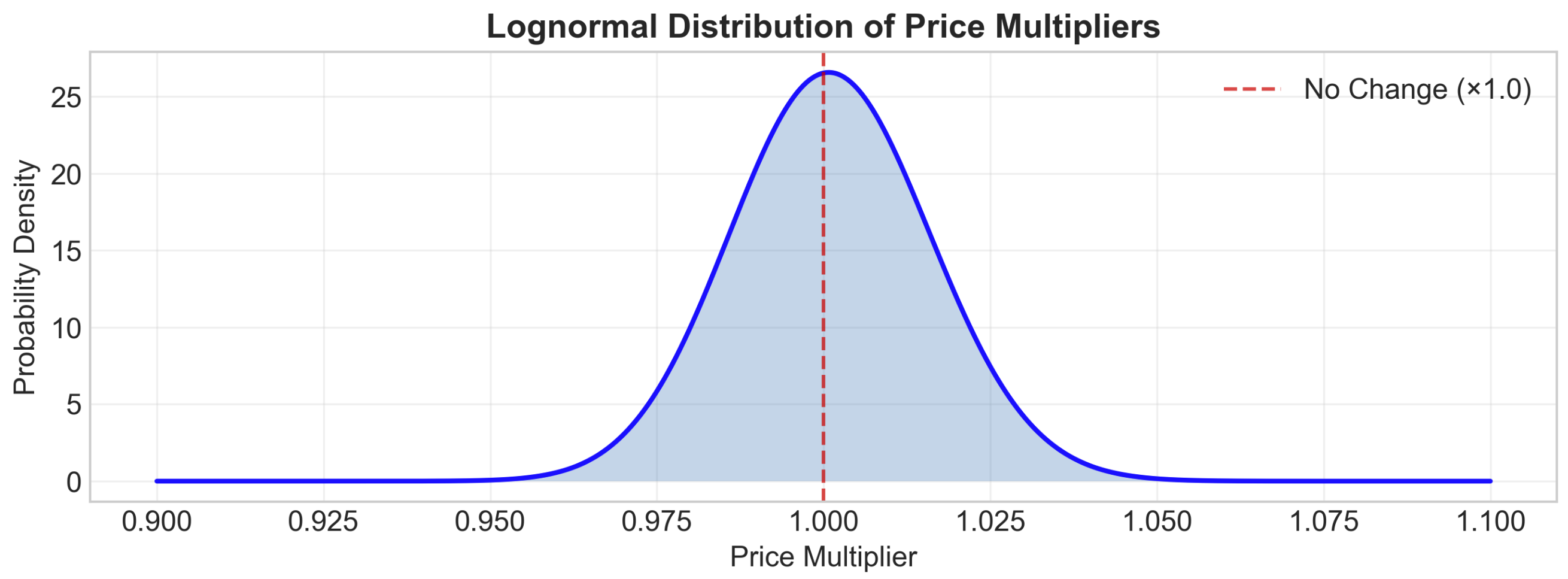
Log Normal Distribution
- Multiplicative Nature of Price Changes: Unlike the normal distribution, which implies that prices change by adding or subtracting fixed amounts, the lognormal distribution models percentage changes. This multiplicative approach aligns with how prices typically evolve in real markets, where changes are often discussed in percentage terms (e.g., "prices increased by 5%").
- Structural Prevention of Negative Values: The lognormal distribution is defined only for positive values, automatically eliminating the possibility of negative prices without requiring additional constraints.
- Asymmetric Distribution: The lognormal distribution features a positive skew, with a long right tail. This asymmetry better captures the reality that price increases can potentially be quite large, while decreases are typically more constrained.
- Natural Handling of Compounding Effects: For long-term forecasts, the lognormal distribution elegantly accommodates the compounding effect of successive price changes, which can lead to exponential growth over extended periods.
Log-Normal - When To Use:
- Long term planningg
- Inlfationary environments
- Financial markets or real assets with potential of appreciation
- Markets with multiplicative dynamics where precentae changes are better descriptors of pricing movements
Calibration of Models
- Validate against previous historical trends
- Reivew Model Sensitivity - how do changes to the model's input parameters effect the projections.
- Domain expterise from knowledabe agents within the field - do the projections make sense to what you are projecting? Do they model real world trends?
- Markets with multiplicative dynamics where precentae changes are better descriptors of pricing movements
Refinements to Models
- Market state shifts - tariffs, government regulation, global economic conditions may have effects
- Revised Correlations - Are there new conditions or information in other analysis that correlate with the model you have built that make it more robust?
- Machine Learning Integation - automate or explan with predictive algoritms.